ANOVA Plot

Plot categorical variable with barplot. Continuous moderator are plotted at ± 1 SD from the mean.

anova_plot(model, predictor = NULL, graph_label_name = NULL, y_lim = NULL)

Arguments

model

fitted model (usually lm or aov object). Variables must be converted to correct data type before fitting the model. Specifically, continuous variables must be converted to type numeric and categorical variables to type factor.

predictor

predictor variable. Must specified for non-interaction plot and must not specify for interaction plot.

graph_label_name

vector or function. Vector should be passed in the form of c(response_var, predict_var1, predict_var2, ...). Function should be passed as a switch function that return the label based on the name passed (e.g., a switch function)

y_lim

the plot's upper and lower limit for the y-axis. Length of 2. Example: c(lower_limit, upper_limit)

Value

a ggplot object

Examples

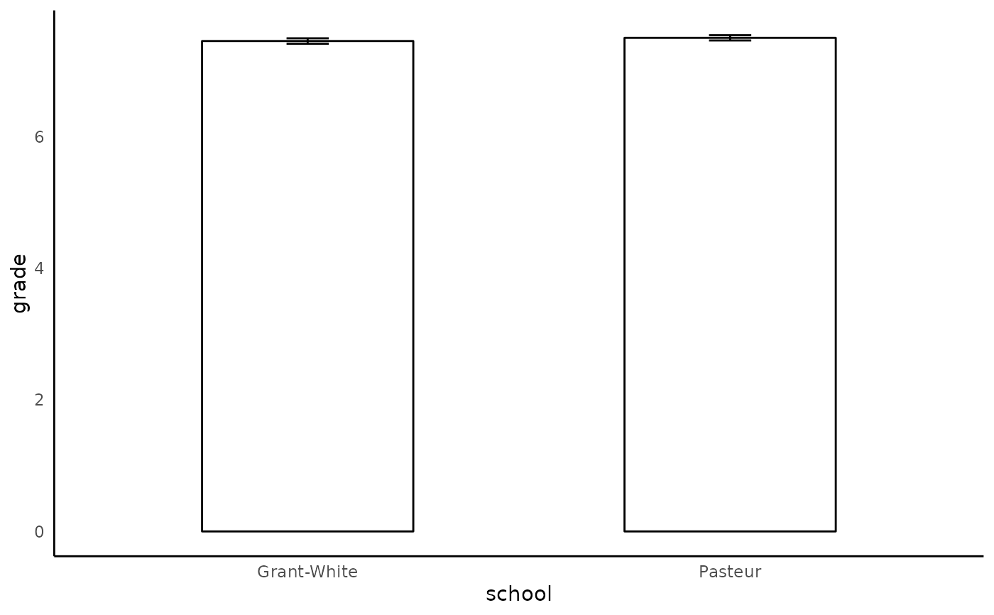
# Main effect plot with 1 categorical variable
fit_1 = lavaan::HolzingerSwineford1939 %>% 
  dplyr::mutate(school = as.factor(school)) %>% 
  lm(data = ., grade ~ school)
anova_plot(fit_1,predictor = school)
#> Loading required namespace: scales
#> Joining with `by = join_by(school)`


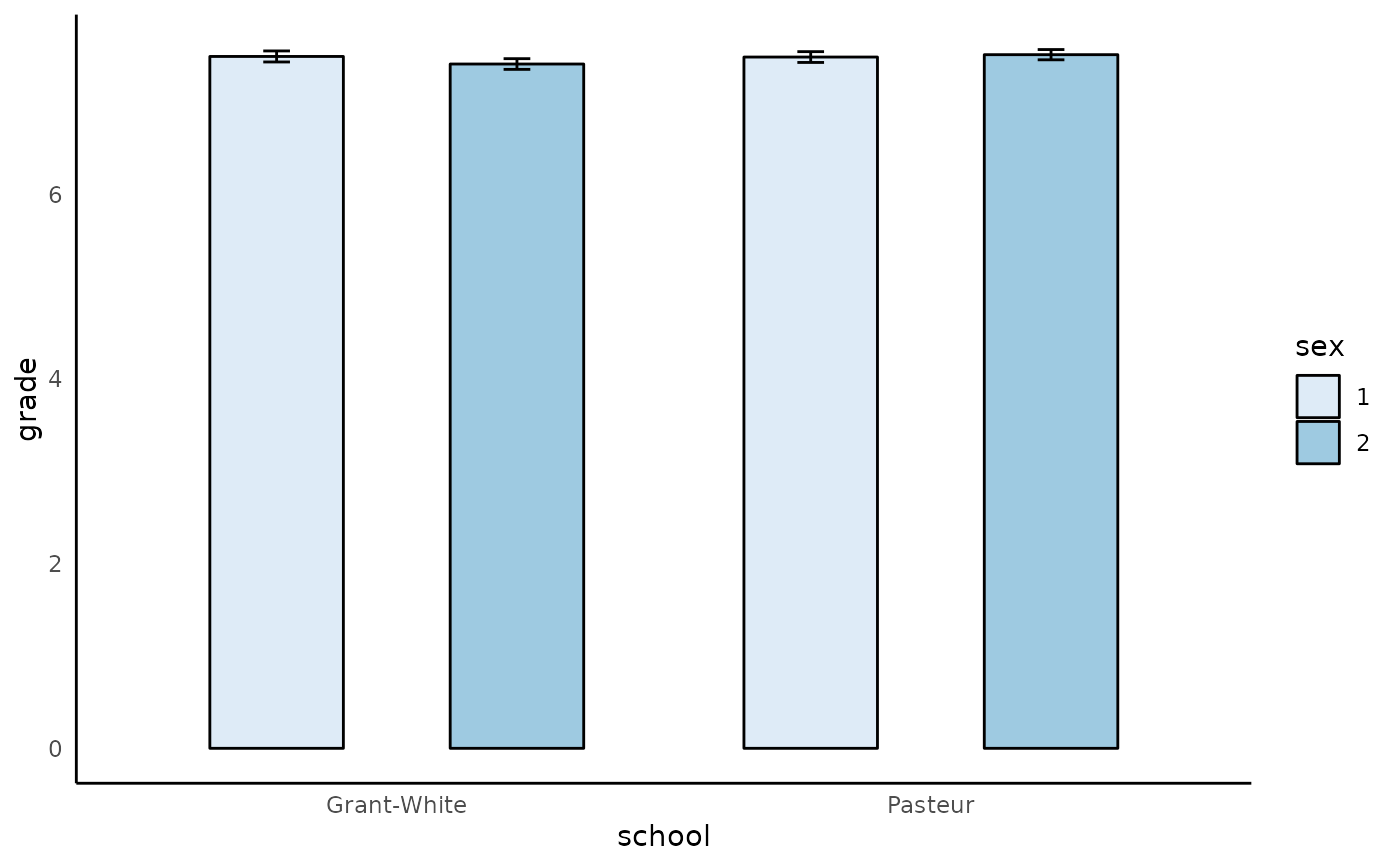
# Interaction effect plot with 2 categorical variables 
fit_2 = lavaan::HolzingerSwineford1939 %>% 
  dplyr::mutate(dplyr::across(c(school,sex),as.factor)) %>% 
  lm(data = ., grade ~ school*sex)
anova_plot(fit_2)
#> Joining with `by = join_by(school, sex)`


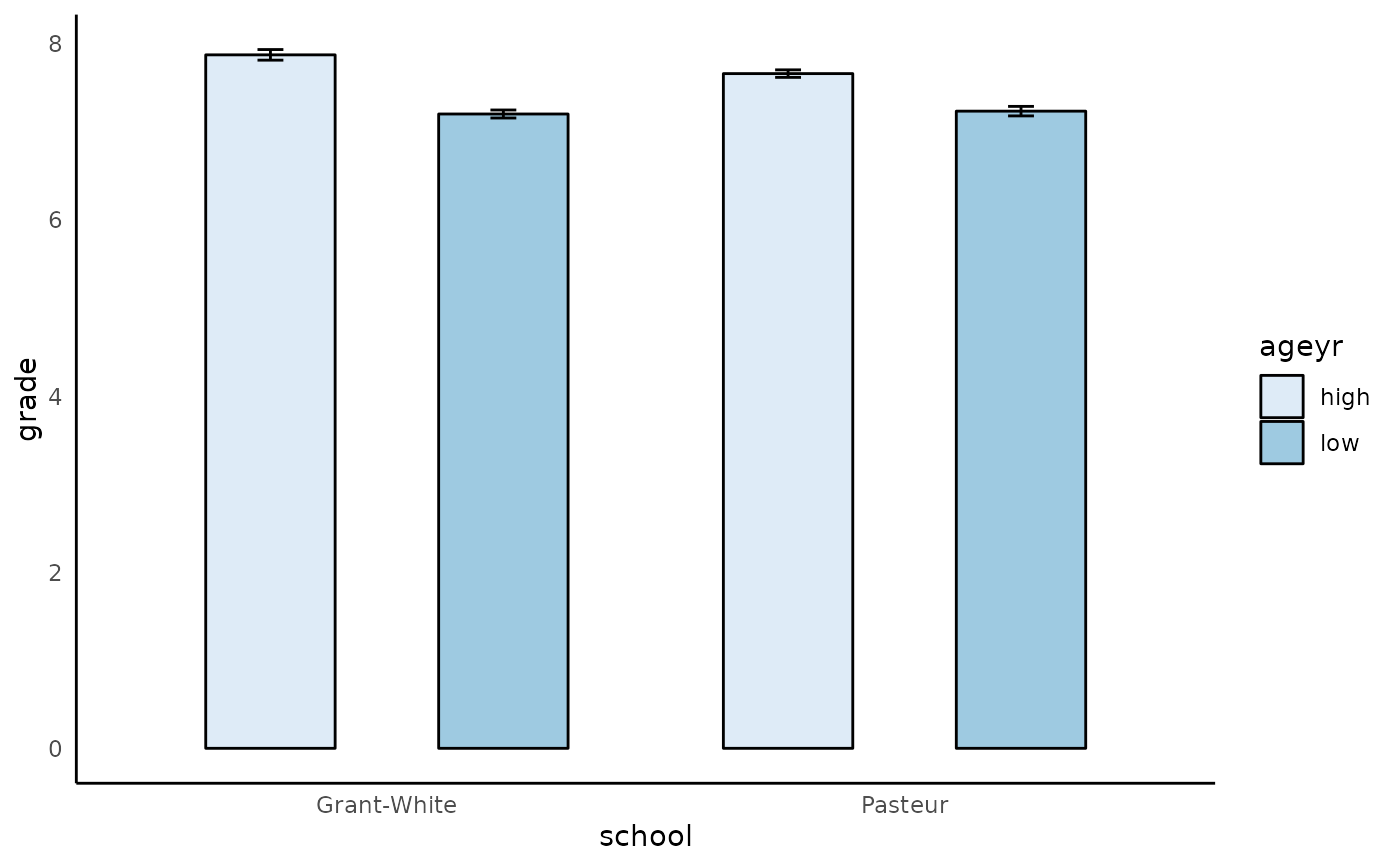
# Interaction effect plot with 1 categorical variable and 1 continuous variable
fit_3 = lavaan::HolzingerSwineford1939 %>% 
  dplyr::mutate(school = as.factor(school)) %>% 
  dplyr::mutate(ageyr = as.numeric(ageyr)) %>% 
  lm(data = ., grade ~ ageyr*school)
anova_plot(fit_3)