Exploratory Factor Analysis — efa

The function is used to fit a exploratory factor analysis model. It will first find the optimal number of factors using parameters::n_factors. Once the optimal number of factor is determined, the function will fit the model using psych::fa(). Optionally, you can request a post-hoc CFA model based on the EFA model which gives you more fit indexes (e.g., CFI, RMSEA, TLI)

efa_summary(
  data,
  cols,
  rotation = "varimax",
  optimal_factor_method = FALSE,
  efa_plot = TRUE,
  digits = 3,
  n_factor = NULL,
  post_hoc_cfa = FALSE,
  quite = FALSE,
  streamline = FALSE,
  return_result = FALSE
)

Arguments

data: data.frame
cols: columns. Support dplyr::select() syntax.
rotation: the rotation to use in estimation. Default is 'oblimin'. Options are 'none', 'varimax', 'quartimax', 'promax', 'oblimin', or 'simplimax'
optimal_factor_method: Show a summary of the number of factors by optimization method (e.g., BIC, VSS complexity, Velicer's MAP)
efa_plot: show explained variance by number of factor plot. default is TRUE.
digits: number of digits to round to
n_factor: number of factors for EFA. It will bypass the initial optimization algorithm, and fit the EFA model using this specified number of factor
post_hoc_cfa: a CFA model based on the extracted factor
quite: suppress printing output
streamline: print streamlined output
return_result: If it is set to TRUE (default is FALSE), it will return a fa object from psych

Value

a fa object from psych

Examples

efa_summary(lavaan::HolzingerSwineford1939, starts_with("x"), post_hoc_cfa = TRUE)
#> 
#>  
#>  
#> Model Summary
#> Model Type = Exploratory Factor Analysis
#> Optimal Factors = 3
#> 
#> Factor Loadings
#> ────────────────────────────────────────────────────────────────
#>   Variable  Factor 1  Factor 3  Factor 2  Complexity  Uniqueness
#> ────────────────────────────────────────────────────────────────
#>         x1               0.613                 1.539       0.523
#>         x2               0.494                 1.093       0.745
#>         x3               0.660                 1.084       0.547
#>         x4     0.832                           1.104       0.272
#>         x5     0.859                           1.043       0.246
#>         x6     0.799                           1.167       0.309
#>         x7                         0.709       1.062       0.481
#>         x8                         0.699       1.131       0.480
#>         x9               0.415     0.521       2.046       0.540
#> ────────────────────────────────────────────────────────────────
#> 
#> 
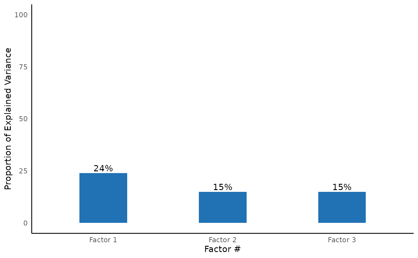
#> Explained Variance
#> ─────────────────────────────────────────────────────
#>                     Var  Factor 1  Factor 3  Factor 2
#> ─────────────────────────────────────────────────────
#>             SS loadings     2.187     1.342     1.329
#>          Proportion Var     0.243     0.149     0.148
#>          Cumulative Var     0.243     0.392     0.540
#>    Proportion Explained     0.450     0.276     0.274
#>   Cumulative Proportion     0.450     0.726     1.000
#> ─────────────────────────────────────────────────────
#> 
#> 
#> EFA Model Assumption Test:
#> OK. Bartlett's test of sphericity suggest the data is appropriate for factor analysis. χ²(36) = 904.097, p < 0.001
#> OK. KMO measure of sampling adequacy suggests the data is appropriate for factor analysis. KMO = 0.752
#> 
#> KMO Measure of Sampling Adequacy
#> ────────────────────
#>       Var  KMO Value
#> ────────────────────
#>   Overall      0.752
#>        x1      0.805
#>        x2      0.778
#>        x3      0.734
#>        x4      0.763
#>        x5      0.739
#>        x6      0.808
#>        x7      0.593
#>        x8      0.683
#>        x9      0.788
#> ────────────────────
#> 

#> 
#> Post-hoc CFA Model Summary
#> 
#> Fit Measure
#> ─────────────────────────────────────────────────────────────────────────────────────
#>       Χ²      DF          P    CFI  RMSEA   SRMR    TLI       AIC       BIC      BIC2
#> ─────────────────────────────────────────────────────────────────────────────────────
#>   85.306  24.000  0.000 ***  0.931  0.092  0.065  0.896  7517.490  7595.339  7528.739
#> ─────────────────────────────────────────────────────────────────────────────────────
#> *** p < 0.001, ** p < 0.01, * p < 0.05, . p < 0.1
#> 
#>  
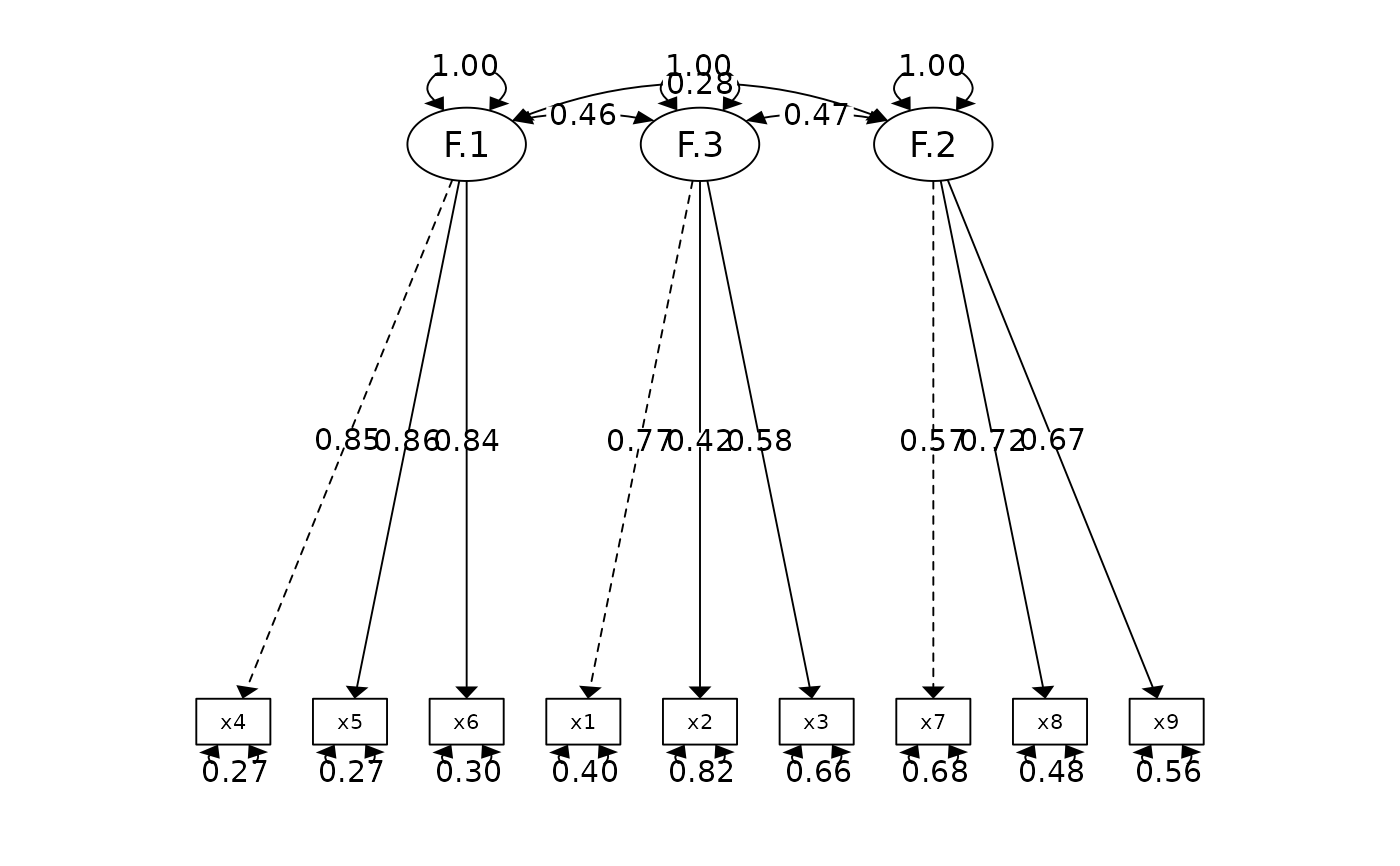
#> Factor Loadings
#> ────────────────────────────────────────────────────────────────────────────────
#>   Latent.Factor  Observed.Var  Std.Est     SE       Z          P          95% CI
#> ────────────────────────────────────────────────────────────────────────────────
#>        Factor.1            x4    0.852  0.023  37.776  0.000 ***  [0.807, 0.896]
#>                            x5    0.855  0.022  38.273  0.000 ***  [0.811, 0.899]
#>                            x6    0.838  0.023  35.881  0.000 ***  [0.792, 0.884]
#>        Factor.3            x1    0.772  0.055  14.041  0.000 ***  [0.664, 0.880]
#>                            x2    0.424  0.060   7.105  0.000 ***  [0.307, 0.540]
#>                            x3    0.581  0.055  10.539  0.000 ***  [0.473, 0.689]
#>        Factor.2            x7    0.570  0.053  10.714  0.000 ***  [0.465, 0.674]
#>                            x8    0.723  0.051  14.309  0.000 ***  [0.624, 0.822]
#>                            x9    0.665  0.051  13.015  0.000 ***  [0.565, 0.765]
#> ────────────────────────────────────────────────────────────────────────────────
#> *** p < 0.001, ** p < 0.01, * p < 0.05, . p < 0.1
#> 
#>  
#> Goodness of Fit:
#>  Warning. Poor χ² fit (p < 0.05). It is common to get p < 0.05. Check other fit measure.
#>  OK. Acceptable CFI fit (CFI > 0.90)
#>  Warning. Poor RMSEA fit (RMSEA > 0.08)
#>  OK. Good SRMR fit (SRMR < 0.08)
#>  Warning. Poor TLI fit (TLI < 0.90)
#>  OK. Barely acceptable factor loadings (0.4 < some loadings < 0.7)