Integrated Function for Linear Regression
integrated_model_summary.Rd![[Stable]](figures/lifecycle-stable.svg)
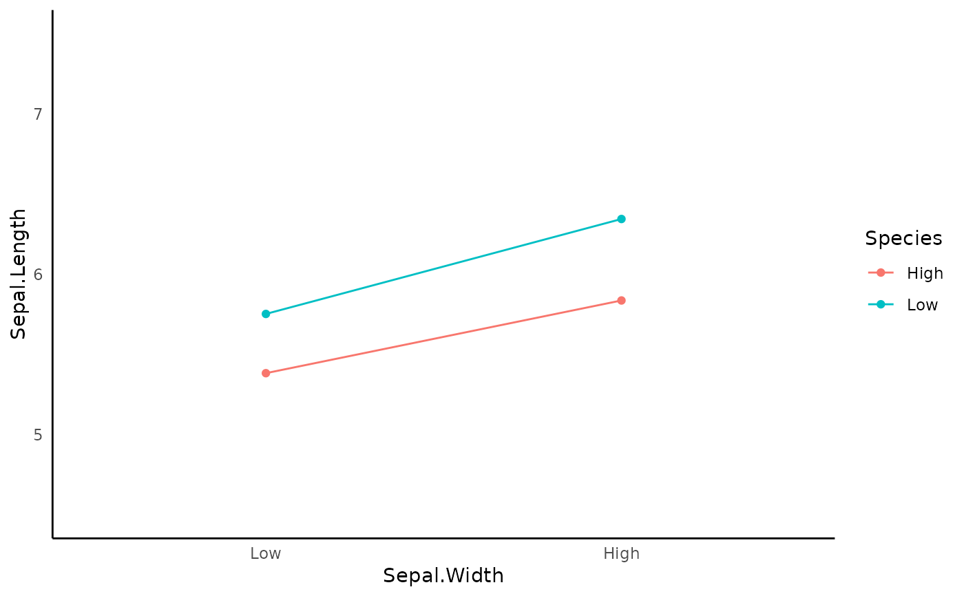
It will first compute the linear regression. Then, it will graph the interaction using the two_way_interaction_plot or the three_way_interaction_plot function.
If you requested simple slope summary, it will calls the interaction::sim_slopes()
integrated_model_summary(
data,
response_variable = NULL,
predictor_variable = NULL,
two_way_interaction_factor = NULL,
three_way_interaction_factor = NULL,
family = NULL,
cateogrical_var = NULL,
graph_label_name = NULL,
model_summary = TRUE,
interaction_plot = TRUE,
y_lim = NULL,
plot_color = FALSE,
digits = 3,
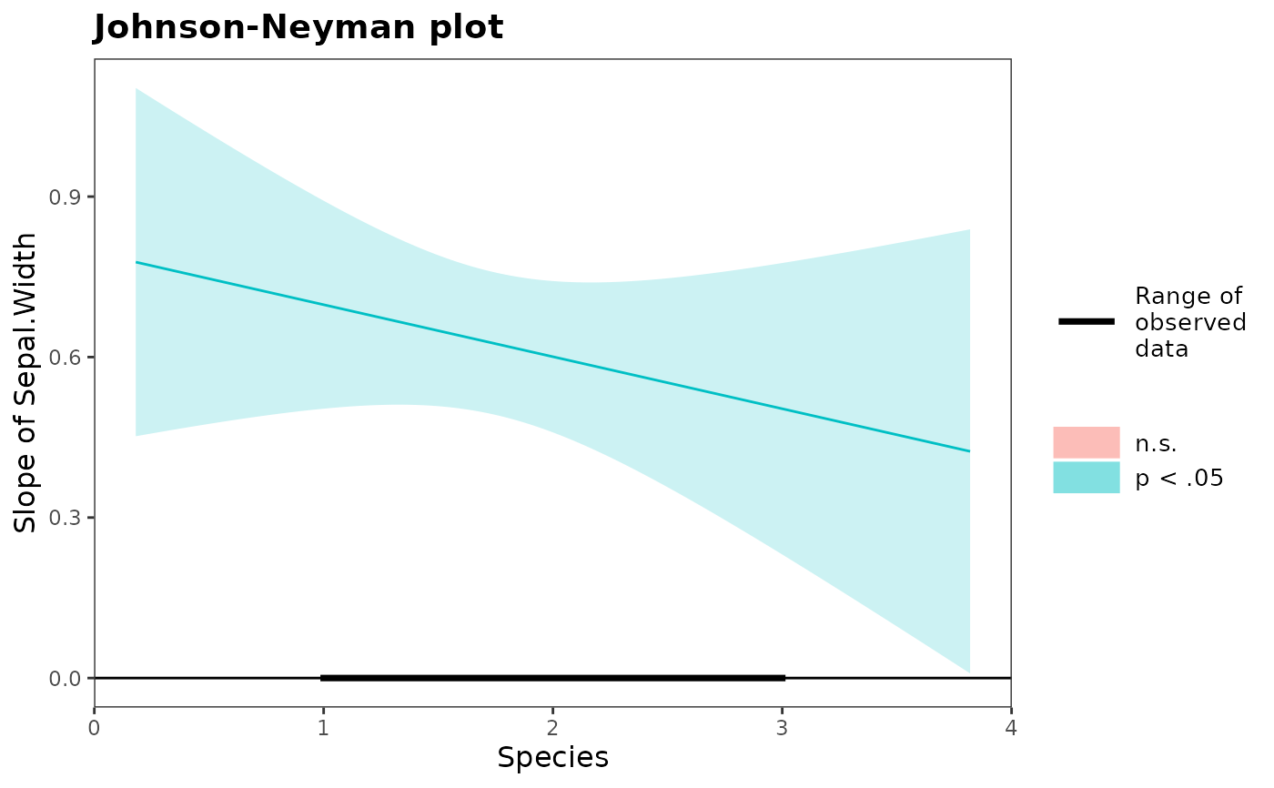
simple_slope = FALSE,
assumption_plot = FALSE,
quite = FALSE,
streamline = FALSE,
return_result = FALSE
)Arguments
- data
data frame
- response_variable
DV (i.e., outcome variable / response variable). Length of 1. Support
dplyr::select()syntax.- predictor_variable
IV. Support
dplyr::select()syntax.- two_way_interaction_factor
two-way interaction factors. You need to pass 2+ factor. Support
dplyr::select()syntax.- three_way_interaction_factor
three-way interaction factor. You need to pass exactly 3 factors. Specifying three-way interaction factors automatically included all two-way interactions, so please do not specify the two_way_interaction_factor argument. Support
dplyr::select()syntax.- family
a GLM family. It will passed to the family argument in glm. See
?glmfor possible options.![[Experimental]](figures/lifecycle-experimental.svg)
- cateogrical_var
list. Specify the upper bound and lower bound directly instead of using ± 1 SD from the mean. Passed in the form of
list(var_name1 = c(upper_bound1, lower_bound1),var_name2 = c(upper_bound2, lower_bound2))- graph_label_name
optional vector or function. vector of length 2 for two-way interaction graph. vector of length 3 for three-way interaction graph. Vector should be passed in the form of c(response_var, predict_var1, predict_var2, ...). Function should be passed as a switch function (see ?two_way_interaction_plot for an example)
- model_summary
print model summary. Required to be
TRUEif you wantassumption_plot.- interaction_plot
generate the interaction plot. Default is
TRUE- y_lim
the plot's upper and lower limit for the y-axis. Length of 2. Example:
c(lower_limit, upper_limit)- plot_color
If it is set to
TRUE(default isFALSE), the interaction plot will plot with color.- digits
number of digits to round to
- simple_slope
Slope estimate at +1/-1 SD and the mean of the moderator. Uses
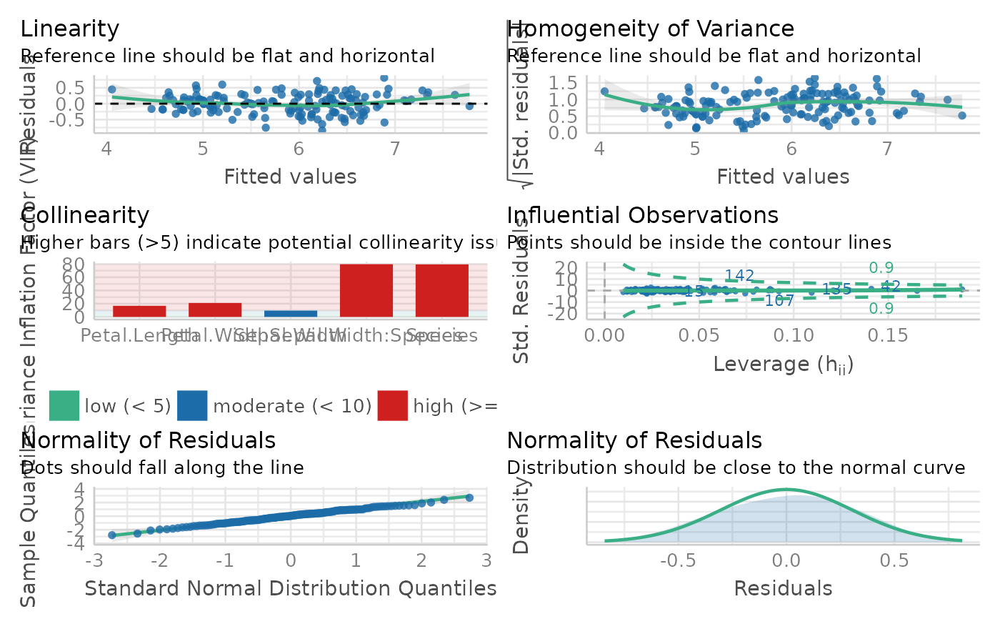
interactions::sim_slope()in the background.- assumption_plot
Generate an panel of plots that check major assumptions. It is usually recommended to inspect model assumption violation visually. In the background, it calls
performance::check_model()- quite
suppress printing output
- streamline
print streamlined output
- return_result
If it is set to
TRUE(default isFALSE), it will return themodel,model_summary, andplot(if the interaction term is included)
Value
a list of all requested items in the order of model, model_summary, interaction_plot, simple_slope
Examples
fit <- integrated_model_summary(
data = iris,
response_variable = "Sepal.Length",
predictor_variable = tidyselect::everything(),
two_way_interaction_factor = c(Sepal.Width, Species)
)
#> Warning: The following columns are coerced into numeric: Species
#>
#>
#> Model Summary
#> Model Type = Linear regression
#> Outcome = Sepal.Length
#> Predictors = Sepal.Width, Petal.Length, Petal.Width, Species
#>
#> Model Estimates
#> ───────────────────────────────────────────────────────────────────────────────────
#> Parameter Coefficient t df SE p 95% CI
#> ───────────────────────────────────────────────────────────────────────────────────
#> (Intercept) 1.552 2.649 144 0.586 0.009 ** [ 0.394, 2.711]
#> Sepal.Width 0.795 4.401 144 0.181 0.000 *** [ 0.438, 1.152]
#> Petal.Length 0.750 12.662 144 0.059 0.000 *** [ 0.633, 0.867]
#> Petal.Width -0.364 -2.370 144 0.154 0.019 * [-0.668, -0.060]
#> Species 0.029 0.105 144 0.278 0.917 [-0.520, 0.578]
#> Sepal.Width:Species -0.097 -1.013 144 0.096 0.313 [-0.287, 0.092]
#> ───────────────────────────────────────────────────────────────────────────────────
#>
#> Goodness of Fit
#> ───────────────────────────────────────────────────
#> AIC BIC R² R²_adjusted RMSE σ
#> ───────────────────────────────────────────────────
#> 83.729 104.803 0.863 0.858 0.305 0.312
#> ───────────────────────────────────────────────────
#>
#> Model Assumption Check
#> OK: Residuals appear to be independent and not autocorrelated (p = 0.998).
#> OK: residuals appear as normally distributed (p = 0.949).
#> Unable to check autocorrelation. Try changing na.action to na.omit.
#> Warning: Heteroscedasticity (non-constant error variance) detected (p = 0.036).
#>
#> Warning: Model has interaction terms. VIFs might be inflated. You may check
#> multicollinearity among predictors of a model without interaction terms.
#> Warning: Severe multicolinearity detected (VIF > 10). Please inspect the following table to identify high correlation factors.
#> Multicollinearity Table
#> ────────────────────────────────────────
#> Term VIF SE_factor
#> ────────────────────────────────────────
#> Sepal.Width 9.518 3.085
#> Petal.Length 16.785 4.097
#> Petal.Width 21.093 4.593
#> Species 79.480 8.915
#> Sepal.Width:Species 79.743 8.930
#> ────────────────────────────────────────
#>
 # \donttest{
fit <- integrated_model_summary(
data = iris,
response_variable = "Sepal.Length",
predictor_variable = tidyselect::everything(),
two_way_interaction_factor = c(Sepal.Width, Species),
simple_slope = TRUE, # you can request simple slope
assumption_plot = TRUE, # you can also request assumption plot
plot_color = TRUE # you can also request the plot in color
)
#> Warning: The following columns are coerced into numeric: Species
#>
#>
#> Model Summary
#> Model Type = Linear regression
#> Outcome = Sepal.Length
#> Predictors = Sepal.Width, Petal.Length, Petal.Width, Species
#>
#> Model Estimates
#> ───────────────────────────────────────────────────────────────────────────────────
#> Parameter Coefficient t df SE p 95% CI
#> ───────────────────────────────────────────────────────────────────────────────────
#> (Intercept) 1.552 2.649 144 0.586 0.009 ** [ 0.394, 2.711]
#> Sepal.Width 0.795 4.401 144 0.181 0.000 *** [ 0.438, 1.152]
#> Petal.Length 0.750 12.662 144 0.059 0.000 *** [ 0.633, 0.867]
#> Petal.Width -0.364 -2.370 144 0.154 0.019 * [-0.668, -0.060]
#> Species 0.029 0.105 144 0.278 0.917 [-0.520, 0.578]
#> Sepal.Width:Species -0.097 -1.013 144 0.096 0.313 [-0.287, 0.092]
#> ───────────────────────────────────────────────────────────────────────────────────
#>
#> Goodness of Fit
#> ───────────────────────────────────────────────────
#> AIC BIC R² R²_adjusted RMSE σ
#> ───────────────────────────────────────────────────
#> 83.729 104.803 0.863 0.858 0.305 0.312
#> ───────────────────────────────────────────────────
#>
#> Model Assumption Check
#> OK: Residuals appear to be independent and not autocorrelated (p = 0.996).
#> OK: residuals appear as normally distributed (p = 0.949).
#> Unable to check autocorrelation. Try changing na.action to na.omit.
#> Warning: Heteroscedasticity (non-constant error variance) detected (p = 0.036).
#>
#> Warning: Model has interaction terms. VIFs might be inflated. You may check
#> multicollinearity among predictors of a model without interaction terms.
#> Warning: Severe multicolinearity detected (VIF > 10). Please inspect the following table to identify high correlation factors.
#> Multicollinearity Table
#> ────────────────────────────────────────
#> Term VIF SE_factor
#> ────────────────────────────────────────
#> Sepal.Width 9.518 3.085
#> Petal.Length 16.785 4.097
#> Petal.Width 21.093 4.593
#> Species 79.480 8.915
#> Sepal.Width:Species 79.743 8.930
#> ────────────────────────────────────────
#> Loading required namespace: qqplotr
#> Loading required namespace: see
# \donttest{
fit <- integrated_model_summary(
data = iris,
response_variable = "Sepal.Length",
predictor_variable = tidyselect::everything(),
two_way_interaction_factor = c(Sepal.Width, Species),
simple_slope = TRUE, # you can request simple slope
assumption_plot = TRUE, # you can also request assumption plot
plot_color = TRUE # you can also request the plot in color
)
#> Warning: The following columns are coerced into numeric: Species
#>
#>
#> Model Summary
#> Model Type = Linear regression
#> Outcome = Sepal.Length
#> Predictors = Sepal.Width, Petal.Length, Petal.Width, Species
#>
#> Model Estimates
#> ───────────────────────────────────────────────────────────────────────────────────
#> Parameter Coefficient t df SE p 95% CI
#> ───────────────────────────────────────────────────────────────────────────────────
#> (Intercept) 1.552 2.649 144 0.586 0.009 ** [ 0.394, 2.711]
#> Sepal.Width 0.795 4.401 144 0.181 0.000 *** [ 0.438, 1.152]
#> Petal.Length 0.750 12.662 144 0.059 0.000 *** [ 0.633, 0.867]
#> Petal.Width -0.364 -2.370 144 0.154 0.019 * [-0.668, -0.060]
#> Species 0.029 0.105 144 0.278 0.917 [-0.520, 0.578]
#> Sepal.Width:Species -0.097 -1.013 144 0.096 0.313 [-0.287, 0.092]
#> ───────────────────────────────────────────────────────────────────────────────────
#>
#> Goodness of Fit
#> ───────────────────────────────────────────────────
#> AIC BIC R² R²_adjusted RMSE σ
#> ───────────────────────────────────────────────────
#> 83.729 104.803 0.863 0.858 0.305 0.312
#> ───────────────────────────────────────────────────
#>
#> Model Assumption Check
#> OK: Residuals appear to be independent and not autocorrelated (p = 0.996).
#> OK: residuals appear as normally distributed (p = 0.949).
#> Unable to check autocorrelation. Try changing na.action to na.omit.
#> Warning: Heteroscedasticity (non-constant error variance) detected (p = 0.036).
#>
#> Warning: Model has interaction terms. VIFs might be inflated. You may check
#> multicollinearity among predictors of a model without interaction terms.
#> Warning: Severe multicolinearity detected (VIF > 10). Please inspect the following table to identify high correlation factors.
#> Multicollinearity Table
#> ────────────────────────────────────────
#> Term VIF SE_factor
#> ────────────────────────────────────────
#> Sepal.Width 9.518 3.085
#> Petal.Length 16.785 4.097
#> Petal.Width 21.093 4.593
#> Species 79.480 8.915
#> Sepal.Width:Species 79.743 8.930
#> ────────────────────────────────────────
#> Loading required namespace: qqplotr
#> Loading required namespace: see
 #>
#> Slope Estimates at Each Level of Moderators
#> ────────────────────────────────────────────────────────────────
#> Species Level Est. S.E. t val. p 95% CI
#> ────────────────────────────────────────────────────────────────
#> Low 0.680 0.087 7.864 0.000 *** [0.509, 0.851]
#> Mean 0.601 0.072 8.392 0.000 *** [0.459, 0.742]
#> High 0.521 0.123 4.236 0.000 *** [0.278, 0.764]
#> ────────────────────────────────────────────────────────────────
#> Note: For continuous variable, low and high represent -1 and +1 SD from the mean, respectively.
#>
#> Slope Estimates at Each Level of Moderators
#> ────────────────────────────────────────────────────────────────
#> Species Level Est. S.E. t val. p 95% CI
#> ────────────────────────────────────────────────────────────────
#> Low 0.680 0.087 7.864 0.000 *** [0.509, 0.851]
#> Mean 0.601 0.072 8.392 0.000 *** [0.459, 0.742]
#> High 0.521 0.123 4.236 0.000 *** [0.278, 0.764]
#> ────────────────────────────────────────────────────────────────
#> Note: For continuous variable, low and high represent -1 and +1 SD from the mean, respectively.
 #> Warning: You requested > 2 plots. Since 1 plot can be displayed at a time, considering using Rmd for better viewing experience.
 # }
# }